Here we’ll analyze the basics of spectral clustering and try to derive it ourselves. I will explain my reasoning behind the functions used and how they operate. The source material notebook is copied from Professor Chodrow’s source.

Clustering

Clusting is important because many times there exist dataset which do not exhibit simple linear trends, but rather are clustered groups. We will use the traditional data analysis packages, and we may import a few more for specific tasks.

import numpy as np
from sklearn import datasets
from matplotlib import pyplot as plt

For our main focus, we will look at two ‘moon’ shaped clusters

np.random.seed(1234)
# number of points to plot
n = 200
# X, is the location of the point. 
# y, is the label designating which cluster it belongs to
X, y = datasets.make_moons(n_samples=n, shuffle=True, noise=0.05, random_state=None)
plt.scatter(X[:,0], X[:,1])

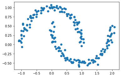
We might theorize that a good way to cluster this data would be to define a small epsilon $e$ and if a point is within epsilon of another point then we will consider them “adjacent”. More on that term soon.

from sklearn.metrics import pairwise_distances 

epsilon = 0.4
A = (pairwise_distances(X, X) < epsilon ).astype(int)
np.fill_diagonal(A, 0) # we define the diagonal to be zero for convience

How can we tell if our labels cluster the data well?

This code takes the “pairwise distance” between every two point and makes a matrix A with entry (i,j) equal to 1 if points i and j are within epsilon of one another. We call it A because it is the Adjacency Matrix. (A term taken from graph theory where two nodes are ‘adjacent’ if they share an edge).

We will take a few other terms from graph theory as well. Such as cut, our next function to introduce. When considering our clusters \(C_0, C_1\), we essentially consider it the number of points near points of a different label.

def cut(A: np.ndarray, y: np.ndarray) -> int:
    total_cut = 0
    # we check every value in the matrix A
    for i in range(len(A)):
        for j in range(len(A)):
            # if i and j are adjacent and they are not the same label add one
            if A[i, j] > 0 and y[i] != y[j]:
                total_cut += 1
    return total_cut/2 # divide by two to avoid double counting

The next function we introduce is the Volume of a cluster. This has a fancy mathematical definition as well, but we will just consider it as a ‘size’ metric. For a cluster \(C_0\) we want to count how many points are adjancent to other points within the same cluster.

from typing import Tuple
def vols(A: np.ndarray, y:np.ndarray) -> Tuple[int]:
    return (A.sum(axis=0)@ (1-y), A.sum(axis=0)@ y)

Now combining those seemingly arbitary functions we can get a mathematical expression \(N_{\mathbf{A}}(C_0, C_1)\equiv \mathbf{cut}(C_0, C_1)\left(\frac{1}{\mathbf{vol}(C_0)} + \frac{1}{\mathbf{vol}(C_1)}\right)\;.\) This expression quantifies how ‘good’ the clusters are separated. Small values of this mean the cut is small (few points in the wrong places) and large volume (clusters are tight).

def normcut(A: np.ndarray, y:np.ndarray) -> int:
    vol_0, vol_1 = vols(A, y)
    return cut(A, y) * (1/vol_0 + 1/vol_1)

Using these we can see that indeed our normcut function gives a small value for the original labels y and a much higher value for some random labels y1.

y1 = np.random.randint(0, 2, len(X))
print(normcut(A, y))
print(normcut(A, y1))

So far, we have been working with the labels given to us. However, our goal is to produce the labels ourself! This means we want the normcut function to be small. Normcut is an inconvient function to work with for computational reasons, so using some hand-wavy linear algebra magic we produce a new vector called \(z \in R^n\) which is defined with the transform function below.

Creating our own labels

def transform(A: np.ndarray, y: np.ndarray) -> np.ndarray:
    vol_0, vol_1 = vols(A, y)
    z = np.vectorize(lambda x: 1/vol_0 if x==0 else -1/vol_1)(y)
    return z

It contains the information of the label as well as giving us the helpful equality, \(\mathbf{N}_{\mathbf{A}}(C_0, C_1) = \frac{\mathbf{z}^T (\mathbf{D} - \mathbf{A})\mathbf{z}}{\mathbf{z}^T\mathbf{D}\mathbf{z}}\;,\)

D = np.diag(A.sum(axis=0))
z = transform(A, y)
print(np.isclose(
    ( z @ (D - A) @ z ) / ( z @ (D) @ z ),
     normcut(A, y)
))

True

Armed with the knowledge of this new function which replicates the ‘good’ metric of clusters, we proceed to optimize this. We use the popular Python module scipy.optimze to allow us to minimize the value of this function. One slight caveat is that we require the vector z to be orthogonal to D1. We provide this code which performs that operation for us.

def orth(u, v):
    return (u @ v) / (v @ v) * v

e = np.ones(n) 

d = D @ e

def orth_obj(z):
    z_o = z - orth(z, d)
    return (z_o @ (D - A) @ z_o)/(z_o @ D @ z_o)

Now let us use the scipy function to find a minimum value for z! The minimize function requires an “initial guess” for what we think our minimum is near, so we’ll provide it a vector of ones.

from scipy.optimize import minimize
z_ = minimize(orth_obj, np.ones(len(z)))
z_min = z_.x
plt.scatter(X[:,0], X[:,1], c = z_min>0)

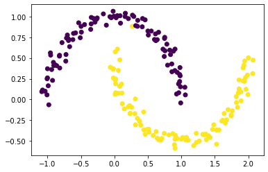
This is really good! We provided a function to optimize, and when minimized, it does labels one cluster as positive values and another as negative values!

What if we aren’t satisfied… What if we have a bigger matrix and scipy is not able to optimize for us! This code we have used to far used 200 points and our computers handled it pretty well, but what if we had 2000 points. Running the code again with 2000 points my computer took over 30 minutes before I stopped it. We’ll need to find another way.

Eigenvectors to the rescue!

Using many handy techniques from linear algebra, we are able to state that the minimum value of our function from above must also be the solution to a certain ‘eigenvector problem’.

Without expounding into too many details about Linear Algebra, essentially we can define a new matrix \(\mathbf{L} = \mathbf{D}^{-1}(\mathbf{D} - \mathbf{A})\). This matrix contains eigenvectors and convieniently we can use the vector corresponding to the second smallest eigenvalue.

The code below using numpy to invert our matrix and to calculate our desired eigenvectors and eigenvalues. Then we select the second smallest and let’s see how it does at labeling our clusters!

L = np.linalg.inv(D) @ (D-A) 
eigenValues, eigenVectors = np.linalg.eig(L)

idx = eigenValues.argsort()   
eigenValues = eigenValues[idx]
eigenVectors = eigenVectors[:,idx]
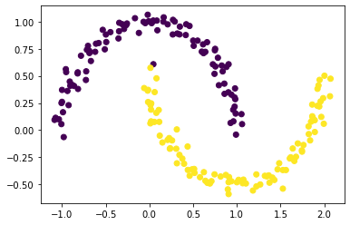
z_eig = eigenVectors[:, 1]
plt.scatter(X[:,0], X[:,1], c = z_eig>0)

Now, lets put it all together to make one special function!

def spectral_clustering(X: np.ndarray, epsilon: int) -> np.ndarray:
    """
    X: vector of shape (n, 2) containing the x and y points of your scattered data
    epsilon: a value to pick to differentiate one cluster from another
    """
    A = (pairwise_distances(X, X) < epsilon ).astype(int) # construct adjacency matrix
    np.fill_diagonal(A, 0)
    D = np.diag(A.sum(axis=0)) # construct diagonal matrix
    L = np.linalg.inv(D) @ (D-A) # construct our linear algebra matrix, L
    eigenValues, eigenVectors = np.linalg.eig(L) # find eigenvalues/vectors
    idx = eigenValues.argsort() # sort
    eigenVectors = eigenVectors[:,idx] # sort
    z_eig = eigenVectors[:, 1] # pick second to last eigenvector
    labels = (z_eig > 0).astype(int) # convert vector to labels of (1's and 0's)
    return labels

Now we can test run this function!

n=1000
X, y = datasets.make_moons(n_samples=n, shuffle=True, noise=0.1, random_state=None)
plt.scatter(X[:,0], X[:,1], c = spectral_clustering(X, epsilon))

Now for a completely new cluster type!

n = 1000
X, y = datasets.make_circles(n_samples=n, shuffle=True, noise=0.05, random_state=None, factor = 0.4)
plt.scatter(X[:,0], X[:,1], c = spectral_clustering(X, 0.3))

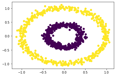
And it works like a charm! We learned a lot