
Blog Post 5 - Tensorflow
We begin our blog post by using the template code provided by Professor Chodrow.
This code initializes the datasets we will use for training and validation of our model.
This code block also uses the tf.data module to speed up the loading of images.
Importing Packages and Dataset
import os
from tensorflow.keras import utils
import tensorflow as tf
import matplotlib.pyplot as plt
from tensorflow.keras.layers import Conv2D, Flatten, Dense, Dropout, MaxPooling2D, InputLayer, ReLU, Softmax, RandomFlip, RandomRotation, Rescaling
# location of data
_URL = 'https://storage.googleapis.com/mledu-datasets/cats_and_dogs_filtered.zip'

# download the data and extract it
path_to_zip = utils.get_file('cats_and_dogs.zip', origin=_URL, extract=True)

# construct paths
PATH = os.path.join(os.path.dirname(path_to_zip), 'cats_and_dogs_filtered')

train_dir = os.path.join(PATH, 'train')
validation_dir = os.path.join(PATH, 'validation')

# parameters for datasets
BATCH_SIZE = 32
IMG_SIZE = (160, 160)

# construct train and validation datasets
train_dataset = utils.image_dataset_from_directory(train_dir,
                                                   shuffle=True,
                                                   batch_size=BATCH_SIZE,
                                                   image_size=IMG_SIZE)

validation_dataset = utils.image_dataset_from_directory(validation_dir,
                                                        shuffle=True,
                                                        batch_size=BATCH_SIZE,
                                                        image_size=IMG_SIZE)

class_names = train_dataset.class_names
# construct the test dataset by taking every 5th observation out of the validation dataset
val_batches = tf.data.experimental.cardinality(validation_dataset)
test_dataset = validation_dataset.take(val_batches // 5)
validation_dataset = validation_dataset.skip(val_batches // 5)

# speed code
AUTOTUNE = tf.data.AUTOTUNE

train_dataset = train_dataset.prefetch(buffer_size=AUTOTUNE)
validation_dataset = validation_dataset.prefetch(buffer_size=AUTOTUNE)
test_dataset = test_dataset.prefetch(buffer_size=AUTOTUNE)
Label Counts
We want to verify we have equal counts of cats and dogs.
# Checking how many of each label exist
labels_iterator = test_dataset.unbatch().map(lambda image, label: label==0).as_numpy_iterator()
sum(labels_iterator)
1000
We see the sum of labels equal to 0 is 1000 out of the 2000 total images, so we expect our baseline to be 0.5 for our predicitions.
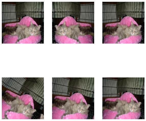
Visualize Images
We also would like to see a sample of some of the images in our dataset to better understand the task. Let’s split the data into two rows, one for cats and one for dogs.
def visualize_images():
    plt.figure(figsize=(10, 10))
    for images, labels in train_dataset.take(1):
        cat_count = 0
        dog_count = 0
        for i in range(len(labels)):
            if class_names[labels[i]] == "cats" and cat_count < 3:
                ax = plt.subplot(2, 3, cat_count + 1)
                plt.imshow(images[i].numpy().astype("uint8"))
                plt.title(class_names[labels[i]])
                plt.axis("off")
                cat_count += 1
                i += 1
            elif class_names[labels[i]] == "dogs" and dog_count < 3:
                ax = plt.subplot(2, 3, dog_count + 4)
                plt.imshow(images[i].numpy().astype("uint8"))
                plt.title(class_names[labels[i]])
                plt.axis("off")
                dog_count += 1
                i += 1

visualize_images()

We see a lot of complexity within these images and so we expect we may need a complicated model to perform precise distinguishing.
Visualizing Training History
We would often like to see how our model trains, so we will make a function to quickly plot the training performance.
def visualize_history(history):
    acc = history.history['accuracy']
    val_acc = history.history['val_accuracy']

    loss = history.history['loss']
    val_loss = history.history['val_loss']

    plt.figure(figsize=(8, 8))
    plt.subplot(2, 1, 1)
    plt.plot(acc, label='Training Accuracy')
    plt.plot(val_acc, label='Validation Accuracy')
    plt.legend(loc='lower right')
    plt.ylabel('Accuracy')
    plt.ylim([min(plt.ylim()),1])
    plt.title('Training and Validation Accuracy')

    plt.subplot(2, 1, 2)
    plt.plot(loss, label='Training Loss')
    plt.plot(val_loss, label='Validation Loss')
    plt.legend(loc='upper right')
    plt.ylabel('Cross Entropy')
    plt.ylim([0,1.0])
    plt.title('Training and Validation Loss')
    plt.xlabel('epoch')
    plt.show()
Model 1
Our first model uses only the initalize 2000 images without any data augmentation or preprocessing. We have a lenient goal of 52% validation accuracy so we imitate a simple model from lecture to hopefully prevent overfitting too much.
# Create our sequntial model similarly to in lecture
model1 = tf.keras.models.Sequential([
    Conv2D(32, 9, activation='relu', input_shape=(160, 160, 3)),
    Dropout(0.3),
    MaxPooling2D((2, 2)),
    Conv2D(32, 6, activation='relu'),
    Dropout(0.3),
    MaxPooling2D((2, 2)),
    Flatten(),
    Dense(64, activation='relu'),
    Dense(1, activation="sigmoid")
])

# Compile using adam optimizer and BinaryCrossentropy loss
model1.compile(optimizer=tf.keras.optimizers.Adam(),
              loss=tf.keras.losses.BinaryCrossentropy(),
              metrics=['accuracy'])

# We train on 20 epochs as prescibed and visualize the training process
history = model1.fit(train_dataset,
                     epochs=20,
                     validation_data=validation_dataset)
visualize_history(history)
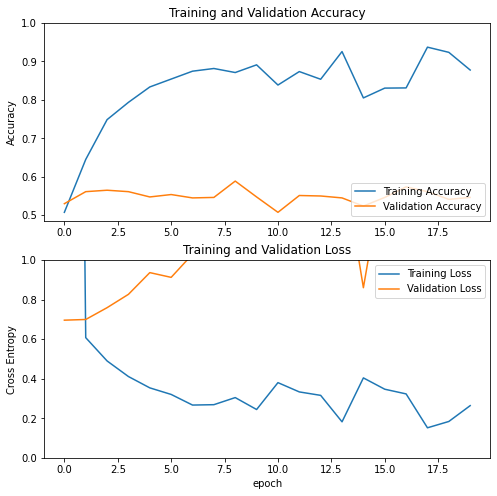
We see gross overfitting and very performance on the validation data, we experimented with many, many other archtectures and all of them tend to overfit. This is due to the very small size of our dataset and the relatively complex task.
Data Augmentation
Data Augmentation is the process of taking exising data and slightly perturbing it in such a way that the distinguishing features stay intact and our model is able to learn on a wider variety of images.
The layers, RandomFlip('horizontal') and RandomRotation(0.1) are layers that we can add to our model which increases the flexibility of training data by flipping and rotating our images respectively. We demonstrate them here:
flipper = tf.keras.Sequential([
    RandomFlip('horizontal')
])
rotater = tf.keras.Sequential([
    tf.keras.layers.RandomRotation(0.1),
])

for image, _ in train_dataset.take(1):
    plt.figure(figsize=(10, 10))
    first_image = image[0]
    # In the first three rows we perform random flips
    for i in range(3):
        ax = plt.subplot(2, 3, i + 1)
        augmented_image = flipper(tf.expand_dims(first_image, 0))
        plt.imshow(augmented_image[0] / 255)
        plt.axis('off')
    # In the second three rows we perform random rotations
    for i in range(3, 6):
        ax = plt.subplot(2, 3, i + 1)
        augmented_image = rotater(tf.expand_dims(first_image, 0))
        plt.imshow(augmented_image[0] / 255)
        plt.axis('off')
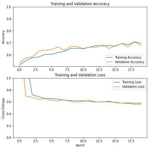
Model 2
By adding data augmentation, we allow ourselves to create a larger model which can better learn distinguishing features.
model2 = tf.keras.Sequential([
    InputLayer(input_shape=(160, 160, 3)),
    # Data Augmentation Layers
    RandomFlip('horizontal'),
    RandomRotation(0.2),

    # Two Sets of Dual Convolutions
    Conv2D(32, 5, activation='relu'),
    Conv2D(32, 3, activation='relu'),
    MaxPooling2D((2, 2)),

    Conv2D(32, 3, activation='relu'),
    Conv2D(32, 3, activation='relu'),
    MaxPooling2D((2, 2)),

    Flatten(),
    # Large Dense layer to learn more features
    Dense(2048, activation='relu'),
    # High Values of Dropout at the end aided in accuracy and overfitting
    Dropout(0.75),
    Dense(1, activation="sigmoid")
])

model2.compile(optimizer=tf.keras.optimizers.Adam(0.0001),
              loss=tf.keras.losses.BinaryCrossentropy(),
              metrics=['accuracy'])

history = model2.fit(train_dataset,
                     epochs=20,
                     validation_data=validation_dataset)
visualize_history(history)
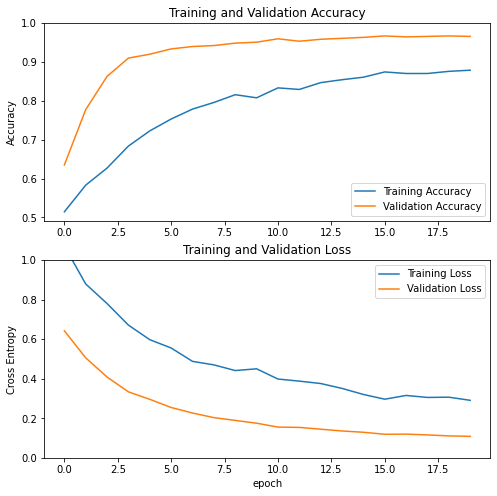
Model 3
The next step in this process will allow us to normalize our image values and let the model parameters also stay within a smaller range. This code block creates a model layer which will process our input images.
i = tf.keras.Input(shape=(160, 160, 3))
x = tf.keras.applications.mobilenet_v2.preprocess_input(i)
preprocessor = tf.keras.Model(inputs = [i], outputs = [x], name='preprocessor')
Now, the relevant model:
model3 = tf.keras.Sequential([
    # Only change is the preprocessor layer
    preprocessor,

    RandomFlip('horizontal'),
    RandomRotation(0.2),

    Conv2D(32, 5, activation='relu'),
    Conv2D(32, 3, activation='relu'),
    MaxPooling2D((2, 2)),

    Conv2D(32, 3, activation='relu'),
    Conv2D(32, 3, activation='relu'),
    MaxPooling2D((2, 2)),

    Flatten(),
    Dense(2048, activation='relu'),
    Dropout(0.75),
    Dense(1, activation="sigmoid")
])

model3.compile(optimizer=tf.keras.optimizers.Adam(0.0001),
              loss=tf.keras.losses.BinaryCrossentropy(),
              metrics=['accuracy'])

history = model3.fit(train_dataset,
                     epochs=20,
                     validation_data=validation_dataset)
visualize_history(history)
 Here we see almost no overfitting and very successful accuracy on validation.
Model 4
Our next model we try is a completely different technique called transfer learning. We will take an exisitng model named MobileNetV2 and fine tune a layer after it to focus on only cats and dogs.
IMG_SHAPE = IMG_SIZE + (3,)
base_model = tf.keras.applications.MobileNetV2(input_shape=IMG_SHAPE,
                                               include_top=False,
                                               weights='imagenet')
base_model.trainable = False

i = tf.keras.Input(shape=IMG_SHAPE)
x = base_model(i, training = False)
base_model_layer = tf.keras.Model(inputs = [i], outputs = [x])
This code allows us to make MobileNetV2 into a frozen layer and insert it into a simple model as below.
model4 = tf.keras.Sequential([
    preprocessor,
    RandomFlip('horizontal'),
    RandomRotation(0.2),

    base_model_layer,
    tf.keras.layers.GlobalAveragePooling2D(),
    Dropout(0.75),
    Dense(1, activation="sigmoid")
])

model4.compile(optimizer=tf.keras.optimizers.Adam(0.0001),
              loss=tf.keras.losses.BinaryCrossentropy(),
              metrics=['accuracy'])

history = model4.fit(train_dataset,
                     epochs=20,
                     validation_data=validation_dataset)
visualize_history(history)
Evaluation on Test Set
Since this fine tuning of MobileNetV2 is by far our best performer we test this on our test dataset.
model4.evaluate(test_dataset)
6/6 [==============================] - 1s 69ms/step - loss: 0.1047 - accuracy: 0.9740
[0.10467348247766495, 0.9739583134651184]
Here we see an accuracy above 97% which is fantastic considering our first models were only getting 60%. However MobileNetV2 is a much more complicated network trained on much more data so it was much more expensive to train. In the end we see that many different CNN architectures exist and there are many techniques to help enable our models to succeed.