
Blog Post 6 - Fake News
In this blog post we will be examining the process of Natural Language Processing using tensorflow through a case study of fake news. These articles were collected in the research paper:
Ahmed H, Traore I, Saad S. (2017) “Detection of Online Fake News Using N-Gram Analysis and Machine Learning Techniques. In: Traore I., Woungang I., Awad A. (eds) Intelligent, Secure, and Dependable Systems in Distributed and Cloud Environments. ISDDC 2017. Lecture Notes in Computer Science, vol 10618. Springer, Cham (pp. 127-138).
Preparation
We begin by retrieving the data prepared by Professor Chodrow cleaned and prepared for us. We will perform additional cleaning shortly.
import pandas as pd
import numpy as np
train_url = "https://github.com/PhilChodrow/PIC16b/blob/master/datasets/fake_news_train.csv?raw=true"
df = pd.read_csv(train_url, header=0, index_col=0)
We check how many of each class there are to ensure the dataset is reasonably distributed.
df.groupby("fake").size()
fake
0 10709
1 11740
dtype: int64
We see there are a similar number of each class. 0 designates if the article is true and 1 designates if the article contains fake news, as determined by the authors of the paper above.
To first clean the data we remove all non-influential ‘words’ as designated by nltk. They maintain a corpus of ‘stop words’ which we can import and remove from our dataset.
# Import stopwords with nltk.
import nltk
nltk.download('stopwords')
from nltk.corpus import stopwords
stop = stopwords.words('english')
Then we create a function to remove these words. Additionally, I also remove any single letter words because my models seemed to be overfitting to these meaningless words.
def rm_stop_words(x: list) -> list:
wd_list = [word for word in x.split() if word not in (stop) + list('abcdefghijklmnopqrstuvwxyz')]
return ' '.join(wd_list)
import tensorflow as tf
def make_dataset(df: pd.DataFrame) -> tf.data.Dataset:
"""
Create new columns by removing the prior words
Create a Tensorflow Dataset object from the pandas Dataframe
Shuffle and Batch the Dataset object
"""
# Applying the previously defined function
df['text_wo_stop'] = df['text'].apply(rm_stop_words)
df['title_wo_stop'] = df['text'].apply(rm_stop_words)
data = tf.data.Dataset.from_tensor_slices(
(
{
"title" : df[["title_wo_stop"]],
"text" : df[["text_wo_stop"]]
},
{
"fake" : df[["fake"]]
}
)
)
# We wish to shuffle the dataset
data = data.shuffle(buffer_size = len(data))
# Using the batch function we group entries
batch = data.batch(20)
return batch
dataset = make_dataset(df)
Now that we have our Tensorflow Dataset object we can begin training. First, we initialize some variables and split our dataset into a train and validation dataset.
DATASET_SIZE = len(dataset)
train_size = int(0.8 * DATASET_SIZE)
val_size = int(0.2 * DATASET_SIZE)
train_dataset = dataset.take(train_size)
val_dataset = dataset.take(val_size)
Now in order to make our model process text we import some layers from tensorflow as well as re for regex and string.
import string
import re
from tensorflow.keras.layers.experimental.preprocessing import TextVectorization
from tensorflow.keras import Input, layers, Model, utils, losses
Using these imports we can make a function to which ‘standarizes’ our string inputs and a layer which vectorizes these inputs.
size_vocabulary = 2000
def standardization(input_data):
lowercase = tf.strings.lower(input_data)
no_punctuation = tf.strings.regex_replace(lowercase,
f"[{re.escape(string.punctuation)}]",
'')
return no_punctuation
vectorize_layer = TextVectorization(
standardize=standardization,
max_tokens=size_vocabulary, # only consider this many words
output_mode='int',
output_sequence_length=500)
vectorize_layer.adapt(train_dataset.map(lambda x, y: x["text"]))
We initialize this layer,
# shared embedding layer
embedding = layers.Embedding(size_vocabulary, 3, name = "embedding")
Models we Used
Model #1 Model with just text input
This model only focuses on the text within each article. We do that by specifying the name in the Input Layer. For now the model will ignore the titles.
text_input = Input(shape = (1,), name = "text", dtype = "string")
# Text Embedding
text_features = vectorize_layer(text_input)
text_features = embedding(text_features)
# Normal Network Architecture
text_features = layers.Dropout(0.2)(text_features)
text_features = layers.GlobalAveragePooling1D()(text_features)
text_features = layers.Dropout(0.2)(text_features)
text_features = layers.Dense(32, activation='relu')(text_features)
output = layers.Dense(1, name = "fake")(text_features)
text_model = Model(
inputs = [text_input],
outputs = output
)
text_model.compile(optimizer = "adam",
loss = losses.BinaryCrossentropy(from_logits=True),
metrics=['accuracy']
)
history = text_model.fit(train_dataset,
validation_data=val_dataset,
epochs = 10,
callbacks=tf.keras.callbacks.EarlyStopping(patience=2))
visualize_history(history)
Epoch 1/10
/usr/local/lib/python3.7/dist-packages/keras/engine/functional.py:559: UserWarning: Input dict contained keys ['title'] which did not match any model input. They will be ignored by the model.
inputs = self._flatten_to_reference_inputs(inputs)
898/898 [==============================] - 6s 6ms/step - loss: 0.4896 - accuracy: 0.6894 - val_loss: 0.2159 - val_accuracy: 0.9333
Epoch 2/10
898/898 [==============================] - 5s 5ms/step - loss: 0.1826 - accuracy: 0.9297 - val_loss: 0.1318 - val_accuracy: 0.9496
Epoch 3/10
898/898 [==============================] - 5s 5ms/step - loss: 0.1280 - accuracy: 0.9550 - val_loss: 0.0958 - val_accuracy: 0.9545
Epoch 4/10
898/898 [==============================] - 5s 6ms/step - loss: 0.1086 - accuracy: 0.9638 - val_loss: 0.0852 - val_accuracy: 0.9808
Epoch 5/10
898/898 [==============================] - 5s 5ms/step - loss: 0.0914 - accuracy: 0.9705 - val_loss: 0.0670 - val_accuracy: 0.9846
Epoch 6/10
898/898 [==============================] - 5s 5ms/step - loss: 0.0843 - accuracy: 0.9711 - val_loss: 0.0590 - val_accuracy: 0.9826
Epoch 7/10
898/898 [==============================] - 5s 5ms/step - loss: 0.0768 - accuracy: 0.9747 - val_loss: 0.0552 - val_accuracy: 0.9868
Epoch 8/10
898/898 [==============================] - 5s 6ms/step - loss: 0.0724 - accuracy: 0.9766 - val_loss: 0.0475 - val_accuracy: 0.9875
Epoch 9/10
898/898 [==============================] - 5s 5ms/step - loss: 0.0624 - accuracy: 0.9797 - val_loss: 0.0435 - val_accuracy: 0.9915
Epoch 10/10
898/898 [==============================] - 5s 6ms/step - loss: 0.0579 - accuracy: 0.9813 - val_loss: 0.0400 - val_accuracy: 0.9888
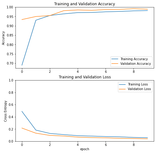
We have good accuracy already! Let’s keep exploring with a similar architecture but focusing on different data.
Model #2 With Just The Title
This model only considers the titles of the articles, similar to the above model.
title_input = Input(shape = (1,), name = "title", dtype = "string")
# Text Embedding
title_features = vectorize_layer(title_input)
title_features = embedding(title_features)
# Normal Network Architecture
title_features = layers.Dropout(0.2)(title_features)
title_features = layers.GlobalAveragePooling1D()(title_features)
title_features = layers.Dropout(0.2)(title_features)
title_features = layers.Dense(32, activation='relu')(title_features)
output = layers.Dense(1, name = "fake")(title_features)
title_model = Model(
inputs = [title_input],
outputs = output
)
title_model.compile(optimizer = "adam",
loss = losses.BinaryCrossentropy(from_logits=True),
metrics=['accuracy']
)
history = title_model.fit(train_dataset,
validation_data=val_dataset,
epochs = 10,
callbacks=tf.keras.callbacks.EarlyStopping(patience=2))
visualize_history(history)
Epoch 1/10
/usr/local/lib/python3.7/dist-packages/keras/engine/functional.py:559: UserWarning: Input dict contained keys ['text'] which did not match any model input. They will be ignored by the model.
inputs = self._flatten_to_reference_inputs(inputs)
898/898 [==============================] - 6s 6ms/step - loss: 0.3751 - accuracy: 0.7962 - val_loss: 0.1499 - val_accuracy: 0.9482
Epoch 2/10
898/898 [==============================] - 5s 5ms/step - loss: 0.1258 - accuracy: 0.9566 - val_loss: 0.0830 - val_accuracy: 0.9679
Epoch 3/10
898/898 [==============================] - 5s 6ms/step - loss: 0.0935 - accuracy: 0.9690 - val_loss: 0.0718 - val_accuracy: 0.9812
Epoch 4/10
898/898 [==============================] - 5s 6ms/step - loss: 0.0812 - accuracy: 0.9747 - val_loss: 0.0632 - val_accuracy: 0.9837
Epoch 5/10
898/898 [==============================] - 5s 6ms/step - loss: 0.0700 - accuracy: 0.9774 - val_loss: 0.0479 - val_accuracy: 0.9877
Epoch 6/10
898/898 [==============================] - 5s 6ms/step - loss: 0.0673 - accuracy: 0.9788 - val_loss: 0.0519 - val_accuracy: 0.9868
Epoch 7/10
898/898 [==============================] - 5s 6ms/step - loss: 0.0604 - accuracy: 0.9806 - val_loss: 0.0424 - val_accuracy: 0.9891
Epoch 8/10
898/898 [==============================] - 5s 6ms/step - loss: 0.0593 - accuracy: 0.9810 - val_loss: 0.0417 - val_accuracy: 0.9913
Epoch 9/10
898/898 [==============================] - 5s 6ms/step - loss: 0.0546 - accuracy: 0.9810 - val_loss: 0.0308 - val_accuracy: 0.9926
Epoch 10/10
898/898 [==============================] - 5s 6ms/step - loss: 0.0523 - accuracy: 0.9833 - val_loss: 0.0349 - val_accuracy: 0.9935
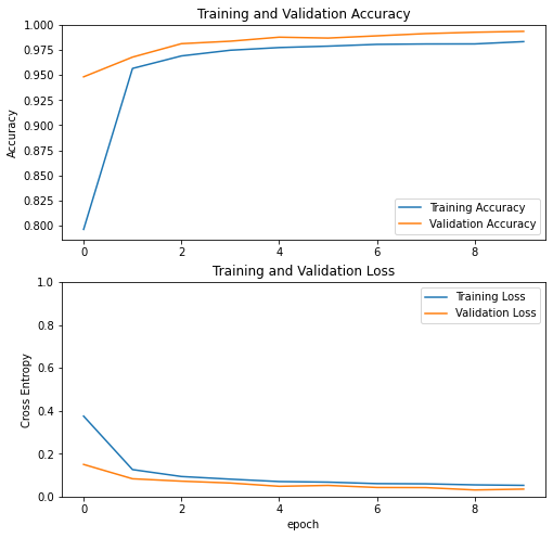
Similar results, it seems our model is still able to recognize content based only on their titles.
Model #3 Combination of Features
combined_features = layers.concatenate([text_features, title_features], axis = 1)
combined_features = layers.Dense(10)(combined_features)
output = layers.Dense(1, name = "fake")(combined_features)
both_model = Model(
inputs = [text_input, title_input],
outputs = output
)
both_model.compile(optimizer = "adam",
loss = losses.BinaryCrossentropy(from_logits=True),
metrics=['accuracy']
)
history = both_model.fit(train_dataset,
validation_data=val_dataset,
epochs = 50,
callbacks=tf.keras.callbacks.EarlyStopping(patience=5))
visualize_history(history)
Epoch 1/50
898/898 [==============================] - 8s 8ms/step - loss: 0.0735 - accuracy: 0.9752 - val_loss: 0.0269 - val_accuracy: 0.9944
Epoch 2/50
898/898 [==============================] - 7s 8ms/step - loss: 0.0417 - accuracy: 0.9888 - val_loss: 0.0259 - val_accuracy: 0.9940
Epoch 3/50
898/898 [==============================] - 7s 8ms/step - loss: 0.0336 - accuracy: 0.9905 - val_loss: 0.0276 - val_accuracy: 0.9933
...
Epoch 27/50
898/898 [==============================] - 7s 8ms/step - loss: 0.0142 - accuracy: 0.9955 - val_loss: 0.0128 - val_accuracy: 0.9964
Epoch 28/50
898/898 [==============================] - 7s 8ms/step - loss: 0.0120 - accuracy: 0.9970 - val_loss: 0.0070 - val_accuracy: 0.9978
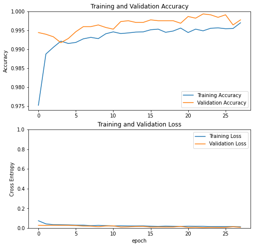
With this combined model and running for at most 50 epochs we get really high (99+%) accuracy now. We can check now how this model performs on the test dataset which we will retrieve from Professor Chodrow’s github.
test_url = "https://github.com/PhilChodrow/PIC16b/blob/master/datasets/fake_news_test.csv?raw=true"
test_df = pd.read_csv(test_url)
test_dataset = make_dataset(test_df)
both_model.evaluate(test_dataset)
1123/1123 [==============================] - 5s 4ms/step - loss: 0.1377 - accuracy: 0.9801
[0.13771803677082062, 0.9800881743431091]
On the test set we get 98% accuracy which is very good! Before we would implement this though we should check to see if there are any intrensic biases.
Weights and Biases
Now that we have a good model, let us analyze how it behaves a bit. We collect the weights associated with each word in our embedding and then we plot a chart to see which words are associated with strong associations in any direction. We copy the lecture notes for this section.
weights = both_model.get_layer('embedding').get_weights()[0] # get the weights from the embedding layer
vocab = vectorize_layer.get_vocabulary() # get the vocabulary from our data prep for later
from sklearn.decomposition import PCA
pca = PCA(n_components=2)
weights = pca.fit_transform(weights)
embedding_df = pd.DataFrame({
'word' : vocab,
'x0' : weights[:,0],
'x1' : weights[:,1]
})
import plotly.express as px
fig = px.scatter(embedding_df,
x = "x0",
y = "x1",
size = list(np.ones(len(embedding_df))),
size_max = 2,
hover_name = "word")
fig.show()
It looks reasonable and as we expect we see political words such as ‘gop’ and ‘trump’ on the far left and right sides.
Next, as in the lecture notes we check for sensitive words to learn about the gender skew of our embedding.
feminine = ["she", "her", "woman"]
masculine = ["he", "him", "man"]
highlight_1 = ["strong", "powerful", "smart", "thinking"]
highlight_2 = ["hot", "sexy", "beautiful", "shopping"]
def gender_mapper(x):
if x in feminine:
return 1
elif x in masculine:
return 4
elif x in highlight_1:
return 3
elif x in highlight_2:
return 2
else:
return 0
embedding_df["highlight"] = embedding_df["word"].apply(gender_mapper)
embedding_df["size"] = np.array(1.0 + 50*(embedding_df["highlight"] > 0))
import plotly.express as px
fig = px.scatter(embedding_df,
x = "x0",
y = "x1",
color = "highlight",
size = list(embedding_df["size"]),
size_max = 10,
hover_name = "word")
fig.show()
Here some of our highlighted words do not even appear in our embedding, and the words we do see are all relatively centered.
Overall, it seems this is model behaves very promisingly on this dataset and in the future we can explore larger datasets and investigate the paper’s designation of fake news to learn more about the subject.